Student's Algorithm for Time-Adjusting Distributions

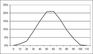
For those readers interest in applied mathematics:

A number of years ago, I was faced with the task of adjusting a distribution of possible outcomes over the life of the relevant phenomenon. I started with two distributions -- a distribution around the mean of possible ultimate outcomes and a time distribution of the expected progression of the mean. Since uncertainty diminishes as time progresses, the distribution of possible outcomes must shrink over time until the ultimate is reached, at which point the distribution of possible outcomes is a single point. The question is how to shrink and adjust the distribution of possible outcomes as time progresses.

I came up with a fairly simple and versatile algorithm to do this that has served me well over the years. I present it here for you. Read more

I. Distributions

D1: Assume the following for the distribution of possible outcomes, with a mean of 60:
10 - 1%, 20 - 2%, 30 - 7%, 40 - 12%, 50 - 18%, 60 - 20%, 70 - 18%, 80 - 12%, 90 - 7%, 100 - 3%


D2: Assume the following for the cumulative time distribution over time, in years:
1- 10%, 2 - 35%, 3 - 80%, 4 - 95%, 5 - 100%

II. Adjusting

What this means is that at time 0, there is a 1% probability that the outcome will be 10 and a 7% that the outcome will be 90. At time 1 (the end of year 1), 10% of the outcome will be known. Therefore, we will know more about the final outcome and the probabilities of the original distribution will have shifted.

How do we account for this additional information? Using the Bornhuetter-Ferguson methodology for the mean, we would take the actual observed (which should be 10% of the ultimate) and add it to the original mean * (100% - 90%). One could apply that to each of the points in D1 but that would require changing the probabilities at which the distribution is evaluated, a task that can become burdensome.

III. Student's Algorithm

Instead, we adjust based on distance from the mean. If the new mean at time 1, using the Born-Ferg methodology, is 55, compared to a mean of 60 at time 0, we look at the distance of each point in the distribution from the mean and apply it to the new mean, reducing it based on D2.

Expected1 = 6. Actual1 = 1. Mean0 = 60. D2,1 = 10%.
Mean1 = Actual1 + (100% - D2,1) * Mean0 = 1 + (100% - 10%) * 60 = 55.

D1 at time 0 looked like this:
10 - 1%, 20 - 2%, 30 - 7%, 40 - 12%, 50 - 18%, 60 - 20%, 70 - 18%, 80 - 12%, 90 - 7%, 100 - 3%

This is now adjusted to take into account the new mean (55) and that 10% of the uncertainty has passed.

The new Point 1 would = Mean1 - (Mean0 - Point1) * (100% - D2,1) = 55 - (60 - 10) * (100% - 10%) = 10 [No change]

The new Point 2 = 55 - (60 - 20) * (100% - 10%) = 19
The new Point 3 = 55 - (60 - 30) * (100% - 10%) = 28

and so on. Here's how the graph looks:


Let's move to time 3 and assume that the actual observed to date is 46. D2,3 = 80% so this should represent 80% of the final outcome. Using Born-Ferg, Mean3 = 46 + (100% - 80%) * 60 = 58.

Since most of the risk has passed, the distribution should have compressed with most of the probability closely surrounding the new mean.

The new point 1 = Mean3 - (Mean0 - Point1) * (100% - D2,3) = 58 - (60 - 10) * (100% - 80%) = 48
The new Point 2 = 58 - (60 - 20) * (100% - 80%) = 50
The new Point 3 = 58 - (60 - 30) * (100% - 80%) = 52
Here's how the graph looks:


Keep doing this at each year end until year 5, where D2 reaches 100% and the distribution is at the single, actual outcome.